Least Squares: Finding the Best Fit#
When you have more equations than unknowns, or when your data is noisy, you can’t always solve \(A\mathbf{x} = \mathbf{b}\) exactly. Instead, you find the best approximate solution using least squares.
The Problem#
Suppose you want to fit a line \(y = mx + c\) to data points that don’t line up perfectly. You want to find \(m\) and \(c\) that minimize the total error.
This is an overdetermined system: more equations (data points) than unknowns (\(m\) and \(c\)).
import numpy as np
import matplotlib.pyplot as plt
Example: Fitting a Line#
Let’s generate some noisy data and fit a line to it:
# Generate noisy data
np.random.seed(42)
x_data = np.linspace(0, 10, 20)
y_true = 2.5 * x_data + 1.5  # True line: y = 2.5x + 1.5
y_data = y_true + np.random.normal(0, 2, size=x_data.shape)  # Add noise

# Plot the data
plt.figure(figsize=(10, 6))
plt.scatter(x_data, y_data, label='Noisy data', alpha=0.6)
plt.plot(x_data, y_true, 'k--', label='True line: y = 2.5x + 1.5', alpha=0.5)
plt.xlabel('x')
plt.ylabel('y')
plt.legend()
plt.title('Noisy Data Points')
plt.grid(True, alpha=0.3)
plt.show()

print(f"We have {len(x_data)} data points but only 2 unknowns (m and c)")
print("This is an overdetermined system!")
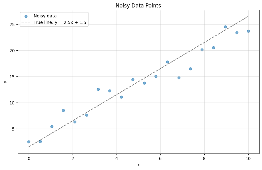
We have 20 data points but only 2 unknowns (m and c)
This is an overdetermined system!
Setting Up the Problem#
For each data point \((x_i, y_i)\), we want:
In matrix form:
Where:
# Build the matrix A and vector b
A = np.column_stack([x_data, np.ones_like(x_data)])
b = y_data

print("Matrix A (first 5 rows):")
print(A[:5])
print(f"\nShape of A: {A.shape}")
print(f"Shape of b: {b.shape}")
print(f"\nWe have {A.shape[0]} equations but only {A.shape[1]} unknowns")
Matrix A (first 5 rows):
[[0.         1.        ]
 [0.52631579 1.        ]
 [1.05263158 1.        ]
 [1.57894737 1.        ]
 [2.10526316 1.        ]]

Shape of A: (20, 2)
Shape of b: (20,)

We have 20 equations but only 2 unknowns
Solving with Least Squares#
The least squares solution minimizes the sum of squared errors:
Use np.linalg.lstsq() to find the best-fit solution:
# Solve using least squares
solution, residuals, rank, singular_values = np.linalg.lstsq(A, b, rcond=None)

m_fit, c_fit = solution

print(f"Best-fit line: y = {m_fit:.3f}x + {c_fit:.3f}")
print(f"True line:     y = 2.500x + 1.500")
print(f"\nTotal squared error: {residuals[0]:.3f}")
Best-fit line: y = 2.122x + 3.049
True line:     y = 2.500x + 1.500

Total squared error: 43.677
Visualizing the Fit#
Let’s plot the data and the fitted line:
# Generate fitted line
y_fit = m_fit * x_data + c_fit

plt.figure(figsize=(10, 6))
plt.scatter(x_data, y_data, label='Data', alpha=0.6, s=50)
plt.plot(x_data, y_true, 'k--', label='True line', alpha=0.5, linewidth=2)
plt.plot(x_data, y_fit, 'r-', label=f'Fitted line: y = {m_fit:.2f}x + {c_fit:.2f}',
         linewidth=2)

# Show residuals (errors)
for i in range(len(x_data)):
    plt.plot([x_data[i], x_data[i]], [y_data[i], y_fit[i]], 'g-', alpha=0.3)

plt.xlabel('x')
plt.ylabel('y')
plt.legend()
plt.title('Least Squares Line Fitting')
plt.grid(True, alpha=0.3)
plt.show()

print("Green lines show the residuals (errors) that are minimized")
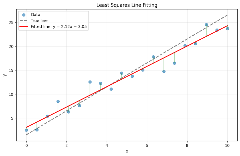
Green lines show the residuals (errors) that are minimized
The Normal Equations#
Mathematically, the least squares solution satisfies the normal equations:
The solution is:
Let’s verify this gives the same answer:
# Solve using normal equations
x_normal = np.linalg.inv(A.T @ A) @ A.T @ b

print("Using lstsq:")
print(f"  m = {m_fit:.6f}, c = {c_fit:.6f}")
print("\nUsing normal equations:")
print(f"  m = {x_normal[0]:.6f}, c = {x_normal[1]:.6f}")
print("\nThey match! But lstsq() is more numerically stable.")
Using lstsq:
  m = 2.121654, c = 3.049133

Using normal equations:
  m = 2.121654, c = 3.049133

They match! But lstsq() is more numerically stable.
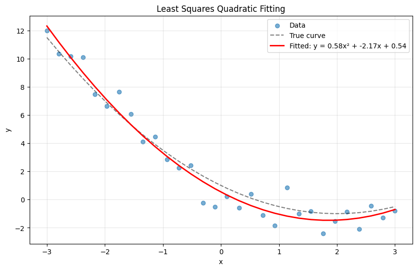
Fitting a Polynomial#
Least squares isn’t limited to straight lines. Let’s fit a quadratic: \(y = ax^2 + bx + c\)
# Generate quadratic data with noise
np.random.seed(42)
x_data = np.linspace(-3, 3, 30)
y_true = 0.5 * x_data**2 - 2 * x_data + 1  # True: y = 0.5x^2 - 2x + 1
y_data = y_true + np.random.normal(0, 1, size=x_data.shape)

# Build matrix for quadratic: [x^2, x, 1]
A_poly = np.column_stack([x_data**2, x_data, np.ones_like(x_data)])

# Solve
coeffs, *_ = np.linalg.lstsq(A_poly, y_data, rcond=None)
a, b, c = coeffs

print(f"Fitted quadratic: y = {a:.3f}x² + {b:.3f}x + {c:.3f}")
print(f"True quadratic:   y = 0.500x² - 2.000x + 1.000")

# Plot
y_fit = a * x_data**2 + b * x_data + c

plt.figure(figsize=(10, 6))
plt.scatter(x_data, y_data, label='Data', alpha=0.6)
plt.plot(x_data, y_true, 'k--', label='True curve', alpha=0.5)
plt.plot(x_data, y_fit, 'r-',
         label=f'Fitted: y = {a:.2f}x² + {b:.2f}x + {c:.2f}', linewidth=2)
plt.xlabel('x')
plt.ylabel('y')
plt.legend()
plt.title('Least Squares Quadratic Fitting')
plt.grid(True, alpha=0.3)
plt.show()
Fitted quadratic: y = 0.585x² + -2.170x + 0.540
True quadratic:   y = 0.500x² - 2.000x + 1.000
NumPy’s Convenience Function#
For polynomial fitting, NumPy provides np.polyfit() as a shortcut:
# Fit a 2nd degree polynomial using polyfit
coeffs_polyfit = np.polyfit(x_data, y_data, deg=2)

print("Using lstsq manually:")
print(f"  [a, b, c] = [{a:.3f}, {b:.3f}, {c:.3f}]")
print("\nUsing np.polyfit:")
print(f"  [a, b, c] = [{coeffs_polyfit[0]:.3f}, {coeffs_polyfit[1]:.3f}, {coeffs_polyfit[2]:.3f}]")
print("\nSame result!")
Using lstsq manually:
  [a, b, c] = [0.585, -2.170, 0.540]

Using np.polyfit:
  [a, b, c] = [0.585, -2.170, 0.540]

Same result!
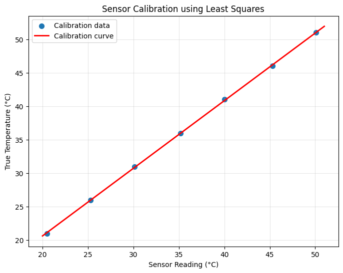
Real-World Example: Sensor Calibration#
Suppose you have a temperature sensor that gives readings, and you want to calibrate it against a reference thermometer:
# Sensor readings vs. true temperatures
sensor_readings = np.array([20.5, 25.3, 30.1, 35.2, 40.0, 45.3, 50.1])
true_temps = np.array([21.0, 26.0, 31.0, 36.0, 41.0, 46.0, 51.0])

# Fit calibration curve: true_temp = m * sensor + c
A_calib = np.column_stack([sensor_readings, np.ones_like(sensor_readings)])
calib_coeffs, *_ = np.linalg.lstsq(A_calib, true_temps, rcond=None)

m_calib, c_calib = calib_coeffs

print(f"Calibration equation: true_temp = {m_calib:.4f} × sensor + {c_calib:.4f}")

# Test it
test_reading = 37.5
calibrated_temp = m_calib * test_reading + c_calib
print(f"\nSensor reads {test_reading}°C")
print(f"Calibrated temperature: {calibrated_temp:.2f}°C")

# Plot calibration
plt.figure(figsize=(8, 6))
plt.scatter(sensor_readings, true_temps, label='Calibration data', s=50)
x_line = np.linspace(20, 51, 100)
y_line = m_calib * x_line + c_calib
plt.plot(x_line, y_line, 'r-', label='Calibration curve', linewidth=2)
plt.xlabel('Sensor Reading (°C)')
plt.ylabel('True Temperature (°C)')
plt.legend()
plt.title('Sensor Calibration using Least Squares')
plt.grid(True, alpha=0.3)
plt.show()
Calibration equation: true_temp = 1.0092 × sensor + 0.4613

Sensor reads 37.5°C
Calibrated temperature: 38.31°C
Summary#
Least squares finds the best approximate solution when \(A\mathbf{x} = \mathbf{b}\) has no exact solution
It minimizes the sum of squared errors: \(\|A\mathbf{x} - \mathbf{b}\|^2\)
Use
np.linalg.lstsq(A, b)for the general caseUse
np.polyfit(x, y, deg)for polynomial fittingThe solution is given by the normal equations: \(\mathbf{x} = (A^T A)^{-1} A^T \mathbf{b}\)
Applications#
Least squares is everywhere:
Curve fitting in data analysis
Linear regression in machine learning
Sensor calibration in engineering
Signal denoising in DSP
Image reconstruction in computer vision
Next Steps#
Now explore how matrices are used in:
Digital Signal Processing - Digital signal processing
Computer Graphics - Computer graphics transformations
Beamforming - Antenna array processing