Solving Systems of Linear Equations

Matrices provide a compact way to solve multiple equations at once. Instead of solving equations one by one, we can solve them all together using matrix operations.

The Problem

Suppose you have a system of linear equations:

\[\begin{split} 2x + 3y &= 8 \\ x - y &= 1 \end{split}\]

We can write this as a matrix equation:

\[ A\mathbf{x} = \mathbf{b} \]

Where:

\[\begin{split} A = \begin{bmatrix} 2 & 3 \\ 1 & -1 \end{bmatrix}, \quad \mathbf{x} = \begin{bmatrix} x \\ y \end{bmatrix}, \quad \mathbf{b} = \begin{bmatrix} 8 \\ 1 \end{bmatrix} \end{split}\]

import numpy as np
import matplotlib.pyplot as plt

Solving with NumPy

NumPy provides np.linalg.solve() to solve \(A\mathbf{x} = \mathbf{b}\):

# Define the system
A = np.array([[2, 3],
              [1, -1]])

b = np.array([8, 1])

# Solve for x
x = np.linalg.solve(A, b)

print(f"Solution: x = {x[0]:.2f}, y = {x[1]:.2f}")

# Verify the solution
print(f"\nVerification:")
print(f"2({x[0]:.2f}) + 3({x[1]:.2f}) = {2*x[0] + 3*x[1]:.2f} (should be 8)")
print(f"({x[0]:.2f}) - ({x[1]:.2f}) = {x[0] - x[1]:.2f} (should be 1)")

Solution: x = 2.20, y = 1.20

Verification:
2(2.20) + 3(1.20) = 8.00 (should be 8)
(2.20) - (1.20) = 1.00 (should be 1)

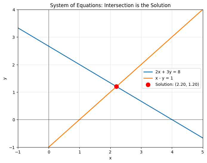
Geometric Interpretation

Each equation represents a line. The solution is where the lines intersect:

# Plot the two equations as lines
x_vals = np.linspace(-2, 6, 100)

# 2x + 3y = 8  =>  y = (8 - 2x) / 3
y1 = (8 - 2*x_vals) / 3

# x - y = 1  =>  y = x - 1
y2 = x_vals - 1

plt.figure(figsize=(8, 6))
plt.plot(x_vals, y1, label='2x + 3y = 8', linewidth=2)
plt.plot(x_vals, y2, label='x - y = 1', linewidth=2)
plt.scatter(x[0], x[1], color='red', s=100, zorder=5, 
            label=f'Solution: ({x[0]:.2f}, {x[1]:.2f})')
plt.xlabel('x')
plt.ylabel('y')
plt.grid(True, alpha=0.3)
plt.axhline(0, color='black', linewidth=0.5)
plt.axvline(0, color='black', linewidth=0.5)
plt.legend()
plt.title('System of Equations: Intersection is the Solution')
plt.xlim(-1, 5)
plt.ylim(-1, 4)
plt.show()

Larger Systems

The same approach works for larger systems. Let’s solve a 3x3 system:

\[\begin{split} x + 2y + z &= 6 \\ 2x + y - z &= 3 \\ x - y + 2z &= 5 \end{split}\]

A = np.array([[1, 2, 1],
              [2, 1, -1],
              [1, -1, 2]])

b = np.array([6, 3, 5])

x = np.linalg.solve(A, b)

print(f"Solution: x = {x[0]:.2f}, y = {x[1]:.2f}, z = {x[2]:.2f}")

# Verify
print(f"\nVerification: A @ x = {A @ x}")
print(f"Should equal b = {b}")
print(f"Difference: {np.linalg.norm(A @ x - b):.2e}")

Solution: x = 2.00, y = 1.00, z = 2.00

Verification: A @ x = [6. 3. 5.]
Should equal b = [6 3 5]
Difference: 0.00e+00

Using the Inverse Matrix

Mathematically, the solution is:

\[ \mathbf{x} = A^{-1}\mathbf{b} \]

Where \(A^{-1}\) is the inverse of \(A\). However, don’t compute the inverse explicitly in practice - np.linalg.solve() is faster and more numerically stable.

A = np.array([[2, 3],
              [1, -1]])
b = np.array([8, 1])

# Using inverse (not recommended)
A_inv = np.linalg.inv(A)
x_inverse = A_inv @ b

# Using solve (recommended)
x_solve = np.linalg.solve(A, b)

print("Using inverse:")
print(f"x = {x_inverse}")
print("\nUsing solve:")
print(f"x = {x_solve}")
print("\nBoth give the same answer, but solve() is better!")

Using inverse:
x = [2.2 1.2]

Using solve:
x = [2.2 1.2]

Both give the same answer, but solve() is better!

When There’s No Solution

If the system has no solution (parallel lines that don’t intersect), the matrix is singular (not invertible):

# Parallel lines: no intersection
A = np.array([[2, 4],
              [1, 2]])  # Second row is half of first row

b = np.array([8, 5])  # Inconsistent right-hand side

try:
    x = np.linalg.solve(A, b)
    print(f"Solution: {x}")
except np.linalg.LinAlgError as e:
    print(f"Error: {e}")
    print("\nThe system has no solution - the lines are parallel!")

# Check if matrix is singular
det = np.linalg.det(A)
print(f"\nDeterminant of A: {det:.2e}")
print("Determinant is zero => matrix is singular")

Error: Singular matrix

The system has no solution - the lines are parallel!

Determinant of A: 0.00e+00
Determinant is zero => matrix is singular

Overdetermined Systems

Sometimes you have more equations than unknowns (e.g., 3 equations, 2 unknowns). This is an overdetermined system and typically has no exact solution.

For these cases, use Least Squares: Finding the Best Fit to find the best approximate solution.

Real-World Example: Circuit Analysis

Solving for currents in an electrical circuit using Kirchhoff’s laws:

\[\begin{split} I_1 + I_2 &= I_3 \quad \text{(current in = current out)} \\ 10I_1 + 5I_2 &= 15 \quad \text{(voltage loop 1)} \\ 5I_2 + 20I_3 &= 25 \quad \text{(voltage loop 2)} \end{split}\]

# Circuit equations in matrix form
A = np.array([[1, 1, -1],
              [10, 5, 0],
              [0, 5, 20]])

b = np.array([0, 15, 25])

I = np.linalg.solve(A, b)

print("Circuit Currents:")
print(f"I1 = {I[0]:.3f} A")
print(f"I2 = {I[1]:.3f} A")
print(f"I3 = {I[2]:.3f} A")

Circuit Currents:
I1 = 1.667 A
I2 = -0.333 A
I3 = 1.333 A

Summary

• Systems of linear equations can be written as \(A\mathbf{x} = \mathbf{b}\)

• Use np.linalg.solve(A, b) to find the solution

• The solution is where all equations (lines/planes) intersect

• If no solution exists, the matrix is singular (determinant = 0)

• For overdetermined systems, use least squares instead

Next Steps

When exact solutions don’t exist, we can still find the best approximate solution using Least Squares: Finding the Best Fit.