Matrix Multiplication

Matrix multiplication is different from element-by-element multiplication. It’s more powerful and represents composition of transformations.

The Key Idea

Matrix multiplication combines two matrices to create a new one. It’s not just multiplying corresponding elements—it involves rows times columns.

For matrices \(A\) (size \(m \times n\)) and \(B\) (size \(n \times p\)), the product \(C = AB\) has size \(m \times p\).

Important: The number of columns in \(A\) must equal the number of rows in \(B\).

The Multiplication Rule

To compute element \((i, j)\) of \(C = AB\):

\[ c_{ij} = \sum_{k=1}^{n} a_{ik} b_{kj} \]

In words: take row \(i\) of \(A\) and column \(j\) of \(B\), multiply corresponding elements, and sum them.

Example

\[\begin{split} \begin{bmatrix} 1 & 2 \\ 3 & 4 \end{bmatrix} \begin{bmatrix} 5 & 6 \\ 7 & 8 \end{bmatrix} = \begin{bmatrix} 1 \cdot 5 + 2 \cdot 7 & 1 \cdot 6 + 2 \cdot 8 \\ 3 \cdot 5 + 4 \cdot 7 & 3 \cdot 6 + 4 \cdot 8 \end{bmatrix} = \begin{bmatrix} 19 & 22 \\ 43 & 50 \end{bmatrix} \end{split}\]

import numpy as np

A = np.array([[1, 2],
              [3, 4]])

B = np.array([[5, 6],
              [7, 8]])

C = A @ B  # Matrix multiplication using @

print("A =")
print(A)
print("\nB =")
print(B)
print("\nA @ B =")
print(C)

A =
[[1 2]
 [3 4]]

B =
[[5 6]
 [7 8]]

A @ B =
[[19 22]
 [43 50]]

Step-by-Step Calculation

Let’s compute each element manually to see how it works:

# Element (0, 0): row 0 of A, column 0 of B
c_00 = A[0, 0] * B[0, 0] + A[0, 1] * B[1, 0]
print(f"c[0,0] = {A[0,0]} * {B[0,0]} + {A[0,1]} * {B[1,0]} = {c_00}")

# Element (0, 1): row 0 of A, column 1 of B
c_01 = A[0, 0] * B[0, 1] + A[0, 1] * B[1, 1]
print(f"c[0,1] = {A[0,0]} * {B[0,1]} + {A[0,1]} * {B[1,1]} = {c_01}")

# Element (1, 0): row 1 of A, column 0 of B
c_10 = A[1, 0] * B[0, 0] + A[1, 1] * B[1, 0]
print(f"c[1,0] = {A[1,0]} * {B[0,0]} + {A[1,1]} * {B[1,0]} = {c_10}")

# Element (1, 1): row 1 of A, column 1 of B
c_11 = A[1, 0] * B[0, 1] + A[1, 1] * B[1, 1]
print(f"c[1,1] = {A[1,0]} * {B[0,1]} + {A[1,1]} * {B[1,1]} = {c_11}")

c[0,0] = 1 * 5 + 2 * 7 = 19
c[0,1] = 1 * 6 + 2 * 8 = 22
c[1,0] = 3 * 5 + 4 * 7 = 43
c[1,1] = 3 * 6 + 4 * 8 = 50

Key Properties

Not Commutative

Important: \(AB \neq BA\) in general. Order matters!

AB = A @ B
BA = B @ A

print("A @ B =")
print(AB)
print("\nB @ A =")
print(BA)
print("\nAre they equal?", np.allclose(AB, BA))

A @ B =
[[19 22]
 [43 50]]

B @ A =
[[23 34]
 [31 46]]

Are they equal? False

Associative

\((AB)C = A(BC)\) — you can group multiplications however you want.

C_mat = np.array([[1, 0],
                  [0, 1]])

# (AB)C
result1 = (A @ B) @ C_mat

# A(BC)
result2 = A @ (B @ C_mat)

print("(A @ B) @ C =")
print(result1)
print("\nA @ (B @ C) =")
print(result2)
print("\nAre they equal?", np.allclose(result1, result2))

(A @ B) @ C =
[[19 22]
 [43 50]]

A @ (B @ C) =
[[19 22]
 [43 50]]

Are they equal? True

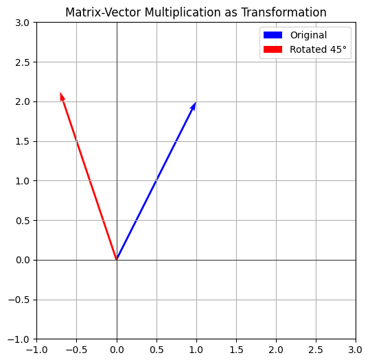
Matrix-Vector Multiplication

A common case: multiply a matrix by a vector. This transforms the vector.

import matplotlib.pyplot as plt

# Original vector
v = np.array([1, 2])

# Transformation matrix (rotation by 45 degrees)
theta = np.pi / 4
R = np.array([[np.cos(theta), -np.sin(theta)],
              [np.sin(theta), np.cos(theta)]])

# Transform the vector
v_transformed = R @ v

print("Original vector:", v)
print("Transformed vector:", v_transformed)

# Visualize
plt.figure(figsize=(6, 6))
plt.quiver(0, 0, v[0], v[1], angles='xy', scale_units='xy', scale=1, 
           color='blue', width=0.006, label='Original')
plt.quiver(0, 0, v_transformed[0], v_transformed[1], angles='xy', 
           scale_units='xy', scale=1, color='red', width=0.006, 
           label='Rotated 45°')
plt.xlim(-1, 3)
plt.ylim(-1, 3)
plt.grid(True)
plt.axhline(0, color='black', linewidth=0.5)
plt.axvline(0, color='black', linewidth=0.5)
plt.legend()
plt.title('Matrix-Vector Multiplication as Transformation')
plt.show()

Original vector: [1 2]
Transformed vector: [-0.70710678  2.12132034]

Why This Definition?

Matrix multiplication is defined this way because it represents composition of linear transformations.

If matrix \(A\) transforms vector \(\mathbf{v}\) to \(A\mathbf{v}\), and matrix \(B\) transforms \(A\mathbf{v}\) to \(B(A\mathbf{v})\), then:

\[ B(A\mathbf{v}) = (BA)\mathbf{v} \]

The product matrix \(BA\) represents doing transformation \(A\) followed by transformation \(B\).

Shape Compatibility

For \(C = AB\):

• \(A\) is \(m \times n\)

• \(B\) is \(n \times p\)

• \(C\) is \(m \times p\)

The inner dimensions must match (\(n\)), and the result has the outer dimensions (\(m \times p\)).

# Example: (2x3) @ (3x4) -> (2x4)
A = np.random.rand(2, 3)
B = np.random.rand(3, 4)
C = A @ B

print(f"A shape: {A.shape}")
print(f"B shape: {B.shape}")
print(f"C = A @ B shape: {C.shape}")

# This would fail:
# D = np.random.rand(2, 5)
# E = A @ D  # Error: shapes (2,3) and (2,5) not aligned

A shape: (2, 3)
B shape: (3, 4)
C = A @ B shape: (2, 4)

Next Steps

Now that you understand matrix multiplication, you can see how matrices represent transformations in Matrices as Transformations.