Matrices as Transformations#
One of the most powerful ways to think about matrices is as transformations of space. When you multiply a matrix by a vector, you’re transforming that vector to a new location.
The Key Insight#
A matrix \(A\) transforms a vector \(\mathbf{v}\) into a new vector \(\mathbf{w}\):
Different matrices perform different transformations: rotations, scalings, reflections, shears, and more.
import numpy as np
import matplotlib.pyplot as plt

def plot_transformation(A, vectors=None, title=""):
    """Plot original and transformed vectors."""
    if vectors is None:
        # Default: unit vectors and a test vector
        vectors = np.array([[1, 0], [0, 1], [1, 1]]).T

    transformed = A @ vectors
    origins = np.zeros(vectors.shape[1])

    fig, (ax1, ax2) = plt.subplots(1, 2, figsize=(12, 5))

    # Original vectors
    ax1.quiver(origins, origins, vectors[0], vectors[1], angles='xy', scale_units='xy',
               scale=1, color=['red', 'blue', 'green'], width=0.006)
    ax1.set_xlim(-3, 3)
    ax1.set_ylim(-3, 3)
    ax1.grid(True, alpha=0.3)
    ax1.axhline(0, color='black', linewidth=0.5)
    ax1.axvline(0, color='black', linewidth=0.5)
    ax1.set_aspect('equal')
    ax1.set_title('Original Vectors')

    # Transformed vectors
    ax2.quiver(origins, origins, transformed[0], transformed[1], angles='xy',
               scale_units='xy', scale=1, color=['red', 'blue', 'green'],
               width=0.006)
    ax2.set_xlim(-3, 3)
    ax2.set_ylim(-3, 3)
    ax2.grid(True, alpha=0.3)
    ax2.axhline(0, color='black', linewidth=0.5)
    ax2.axvline(0, color='black', linewidth=0.5)
    ax2.set_aspect('equal')
    ax2.set_title('Transformed Vectors')

    if title:
        fig.suptitle(title, fontsize=14, fontweight='bold')

    plt.tight_layout()
    plt.show()
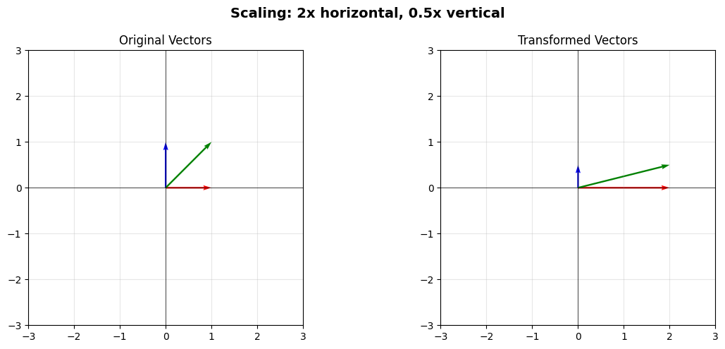
Scaling#
A diagonal matrix scales vectors along each axis:
This doubles the \(x\)-component and halves the \(y\)-component.
# Scaling matrix
S = np.array([[2, 0],
              [0, 0.5]])

print("Scaling matrix:")
print(S)

plot_transformation(S, title="Scaling: 2x horizontal, 0.5x vertical")
Scaling matrix:
[[2.  0. ]
 [0.  0.5]]
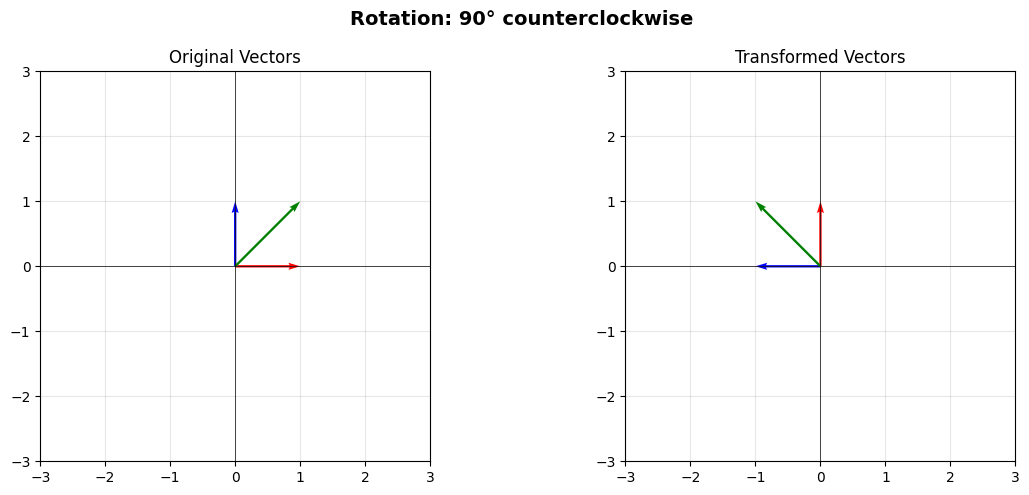
Rotation#
A rotation matrix rotates vectors by an angle \(\theta\):
Let’s rotate by 90 degrees (\(\pi/2\) radians):
# 90 degree rotation
theta = np.pi / 2
R = np.array([[np.cos(theta), -np.sin(theta)],
              [np.sin(theta), np.cos(theta)]])

print("Rotation matrix (90°):")
print(R)

plot_transformation(R, title="Rotation: 90° counterclockwise")
Rotation matrix (90°):
[[ 6.123234e-17 -1.000000e+00]
 [ 1.000000e+00  6.123234e-17]]
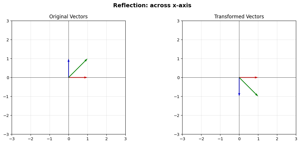
Reflection#
Reflection across the \(x\)-axis flips the \(y\)-coordinate:
# Reflection across x-axis
F = np.array([[1, 0],
              [0, -1]])

print("Reflection matrix:")
print(F)

plot_transformation(F, title="Reflection: across x-axis")
Reflection matrix:
[[ 1  0]
 [ 0 -1]]
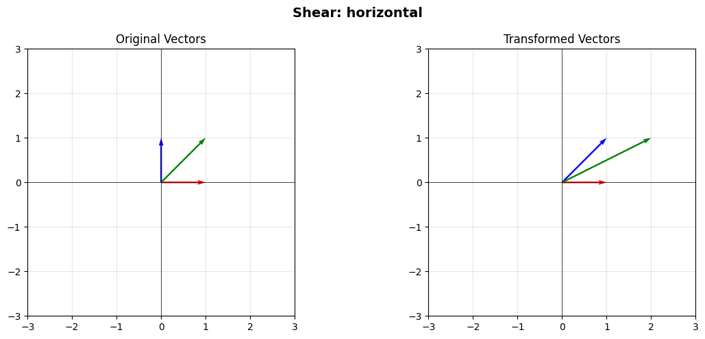
Shear#
A shear transformation “skews” space:
This adds the \(y\)-coordinate to the \(x\)-coordinate, creating a slant.
# Horizontal shear
H = np.array([[1, 1],
              [0, 1]])

print("Shear matrix:")
print(H)

plot_transformation(H, title="Shear: horizontal")
Shear matrix:
[[1 1]
 [0 1]]
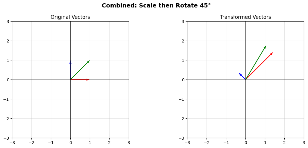
Composing Transformations#
You can combine transformations by multiplying matrices. The order matters!
Let’s rotate by 45° and then scale:
# Rotation by 45 degrees
theta = np.pi / 4
R45 = np.array([[np.cos(theta), -np.sin(theta)],
                [np.sin(theta), np.cos(theta)]])

# Scaling
S = np.array([[2, 0],
              [0, 0.5]])

# Combined: scale THEN rotate
combined = R45 @ S

print("Combined transformation (rotate after scale):")
print(combined)

plot_transformation(combined, title="Combined: Scale then Rotate 45°")
Combined transformation (rotate after scale):
[[ 1.41421356 -0.35355339]
 [ 1.41421356  0.35355339]]
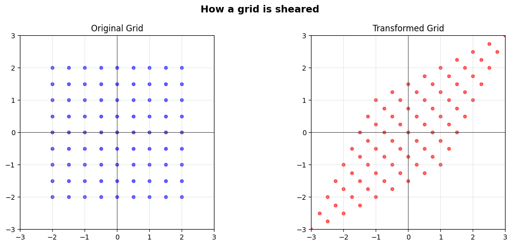
Transforming the Grid#
Let’s visualize how a transformation affects an entire grid of points:
def plot_grid_transformation(A, title=""):
    """Plot how a grid is transformed."""
    # Create a grid of points
    x = np.linspace(-2, 2, 9)
    y = np.linspace(-2, 2, 9)
    X, Y = np.meshgrid(x, y)

    # Flatten to column vectors
    points = np.vstack([X.ravel(), Y.ravel()])

    # Transform
    transformed = A @ points

    fig, (ax1, ax2) = plt.subplots(1, 2, figsize=(12, 5))

    # Original grid
    ax1.scatter(points[0], points[1], c='blue', s=20, alpha=0.6)
    ax1.set_xlim(-3, 3)
    ax1.set_ylim(-3, 3)
    ax1.grid(True, alpha=0.3)
    ax1.axhline(0, color='black', linewidth=0.5)
    ax1.axvline(0, color='black', linewidth=0.5)
    ax1.set_aspect('equal')
    ax1.set_title('Original Grid')

    # Transformed grid
    ax2.scatter(transformed[0], transformed[1], c='red', s=20, alpha=0.6)
    ax2.set_xlim(-3, 3)
    ax2.set_ylim(-3, 3)
    ax2.grid(True, alpha=0.3)
    ax2.axhline(0, color='black', linewidth=0.5)
    ax2.axvline(0, color='black', linewidth=0.5)
    ax2.set_aspect('equal')
    ax2.set_title('Transformed Grid')

    if title:
        fig.suptitle(title, fontsize=14, fontweight='bold')

    plt.tight_layout()
    plt.show()

# Try with a shear transformation
H = np.array([[1, 0.5],
              [0.5, 1]])

plot_grid_transformation(H, title="How a grid is sheared")
The Identity Matrix#
The identity matrix \(I\) leaves vectors unchanged:
It’s the “do nothing” transformation.
I = np.eye(2)

v = np.array([2, 3])
result = I @ v

print(f"I @ {v} = {result}")
print("\nThe identity matrix leaves vectors unchanged.")
I @ [2 3] = [2. 3.]

The identity matrix leaves vectors unchanged.
Why This Matters#
Thinking of matrices as transformations is incredibly powerful:
Computer Graphics: Every 3D rotation, translation, and projection is a matrix
Robotics: Transforming coordinates between robot joints
Data Science: PCA and dimensionality reduction are geometric transformations
Physics: State transformations in quantum mechanics
When you see matrix multiplication, think: “What transformation is happening here?”
Next Steps#
Now that you understand matrices as transformations, you’re ready to explore:
Solving Systems of Linear Equations - Using matrices to solve equations
Least Squares: Finding the Best Fit - Finding best-fit solutions
Applications in graphics, signal processing, and engineering